Galaxy formation models

• Galaxy formation models - general framework of gravitational instability models. Distinction between dissipationless and dissipational collapse. Former applies to DM, latter to baryonic; clearly need to understand baryonic to predict galaxies, but since gravity may be dominated by DM, must understand dissipationless collapse first.

• Main components:
  • Initial conditions
  • Dark matter evolution
  • Gas evolution
  • Star formation and compact object formation
  • Feedback: stellar and black hole
  • Merging

• Challenges:
  • Large dynamic range: stars ($\sim 1Msun$) to galaxy clusters ( $\sim 10^{15} Msun$), structure on sub-pc to 100 Mpc scales
  • Cosmological model uncertainty: but this is converging, and it is a model where merging is important, so evolution of objects cannot be considered in isolation
  • Lack of knowledge of detailed physics of black hole formation and star formation
  • Lack of knowledge of detailed physics of feedback
  • Because of challenges, neither full numerical nor full analytical analysis is possible

• Initial conditions
  • Determined from early Universe physics + cosmological model
  • Can be calculated analytically so long as perturbations are linear (small).
  • Initial spectrum of perturbations from inflationary era: characterized by spectrum of density perturbations:
    
    $$\delta_k = {1\over V}\int d^3x \delta(x)e^{ik\dot x}$$
    
    
    where $\delta(x)$ is overdensity at different locations. Inflation predictes $\delta_k \propto k$ (Harrison-Zeldovich spectrum)
  • Perturbations grow when they become causally connected (cross the horizon)
  • Early in Universe history, radiation density ( $\rho_r \propto a^{-4}$) dominated matter density ( $\rho_m \propto a^{-3}$). Suppresses growth of smaller perturbations.
  • Early in Universe, matter was ionized, leading to strong coupling between baryons and radiation. Prevents growth of baryonic perturbations, and leaves imprint of acoustic oscillations
  • After recombination, baryons fall into dark matter perturbations
  • These processes imprint characteristic perturbation spectrum that can be used for initial conditions
  • Normalization of spectrum not predicted a priori, however; often characterized by $\sigma_8$: rms mass perturbations on $8h^{-1}$ Mpc scale, and constrained by various large scale structure observations.

• Dark matter evolution
  • Can be calculated numerically, e.g. by N-body simulations. Large dynamic range poses challenges for direct summation. Various techniques used to yield results.
  • Perturbation spectrum has smaller halos collapsing first on average, but with significant overlap in collapse times for halos of different scales.
  • As time progresses, significant merging of halos occurs
  • Growth of dark matter halos has also been studied using semi-analytic models, e.g. Bond et al., Lacy & Cole, etc. These take realization of initial perturbation spectrums and produce histories of mergers/accretion for objects of different masses
  • Present day dark matter halos characterized by their mass accretion history (MAH)
  • Dark matter halos found to have characteristic density profiles, often described by the Navarro-Frenk-White (NFW) profile ( $\propto r^{-1}$ in inner regions, $\propto r^{-3}$ in outer regions. Transition radius varies for halos of different masses, charactized by the halo concentration
  • Dark matter halos have some angular momentum; distribution of angular momentum often characterized by distribution of dimensionless spin parameter, $\lambda$

• Gas evolution
  • Gas moves in dark matter potentials, but also has pressure, and can cool, shock, etc.
  • Numerical hydrodynamical simulations becoming more and more feasible. Various techniques used, e.g. smoothed particle hydrodynamics (SPH), adaptive mesh refinefine (AMR)
  • Gas collapses when cooling time becomes short compared to dynamical time, happens quicker at higher densities and lower temperatures. Cooling time is relatively short in inner parts of halos, slower in outer parts
  • Various ``semi-analytical'' schemes have been developed to estimate rate of mass accretion in different dark matter halos, based on cooling time arguments, etc., e.g. White & Frenk 1991
  • Details of cooling are more complex, c.f. numerical simulations, where gas accretes along filaments, and not at all spherically

• Star formation
  • Lacking detailed knowledge of star formation, and lack of sufficient resolution, star formation is paratemeterized within models, e.g. based on stability arguments given gas densities and temperatures
  • Parameterization tuned by need to match charactertic observed relations of observed star formation, e.g. Kennicutt law

• Feedback
  • mass function of dark matter halos differs significantly from mass function of galaxies, suggesting there are processes that suppress galaxy formation at low and high galaxy masses
  • one finds that gas cools and forms stars in small galaxies early (the ``cooling catastrophe'') and cannot build up big galaxies
  • one also finds that gas may collapse too much in halos, leading to galaxies that are too small compared with real galaxies
  • These problems have suggested the importance of feedback, i.e. energy deposition back into gas
    • Energy from stars within galaxies via stellar winds and supernovae
    • Energy from massive black holes
    • Energy from surrouding galaxy population, e.g. significant UV flux to cause photoionization

• Merging
  • While merging of dark matter halos can be followed using the dark matter simulations, merging of galaxies within halos procedes at a slower rate, because they are centrally condensed
  • Merging is increased within a common dark matter halo by the process of dynamical friction, which transfers angular momentum from orbiting objects to dark halo
  • Merging of galaxies may be important in triggering, and subsequently cutting off star formation

• Semi-analytic models
  • Given various uncertain input physics and parameterizations thereof, may be productive to use ``semi-analytic'' models to compare with observed galaxy population
  • Initial semi-analytic models done using semi-analytic merging trees, cooling, star formation, and feedback
  • More recent semi-analytic models, e.g. the Millenium simulation, use numerical dark matter simulations to produce spatial halo distribution with mass accretion histories for each halo, then add semi-analytic cooling, star formation and feedback; these have the advantage of giving large scale environment
  • Semi-analytic models starting to reproduce observed luminosity function, color-bimodality of galaxies, mass-metallicity relation, Tully-Fisher relation, etc. fairly well. See figures in Croton et al, MNRAS 365, 11 (2006)

• Numerical models
  • Numerical models attempt to capture gas physics more accurately
  • they also provide internal structure of galaxies
  • realistic galaxies starting to appear in such simulations, but not yet possible to do large numbers of individual galaxies within large simulation volumes

Growth of perturbations in expanding universe for cold particles, within horizon

Consider analogy to growth of perturbation by gravity in expanding universe to that in Euclidean space.

General behavior as f($\Omega$): $\Omega\geq 1$, growth continues forever, $\Omega<1$, growth stops at $(1+z)\sim 1/\Omega$. Sketch rough curve for growth of a perturbation. Schematically sketch a perturbation and discuss relation between density of perturbation and mass of pertubation.

Growth of spherical perturbation can be solved analytically. Here, we simply sketch out some of the main results for the simple case of spherical perturbations and $\Omega=1$ ; full derivations are not shown, and remember, the preferred current cosmological model does not have $\Omega=1$ !.

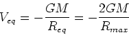
Growth rate given by Birchoff's theorem of GR ( external matter exerts no force):

$${d^2R\over dt^2} = -{GM\over R^2} = -{4\pi G\over 3}\rho(1+\delta)R$$

where we've defined the overdensity, $\delta$. This applies to spherical perturbation. This can be compared with equation for evoltuion of scale factor of the univers

$${d^2a\over dt^2} = -{GM\over a^2} = -{4\pi G\over 3}\rho a$$

Consequently, perturbation with amplitude $\delta$ just grows like universe with different $\Omega$. Integrating equation once, we get

$${1\over 2} ({dR\over dt})^2 - {GM\over R} = E(M)$$

where $E(M)$ is a constant which is the total energy. Evaluating at maximum expansion radius, we get

$$E(M) = -{GM\over R_{max}}$$

Integrating once more, we get

$$t(R) = \int_0^R dr ({2GM\over r} - {2GM\over R_{max}})^{-1/2}$$

which, for a perturbation at early times, when $r«R_{max}$, gives

$$t\propto R^{3/2}$$

$$R\propto t^{2/3}$$

As perturbation grows, this growth rate slows down - can write solution parametrically (not here), similarly to equations for closed and open universes. For the whole universe, $R_{max}=\infty$ for $\Omega=1$, and

$$a\propto t^{2/3}$$

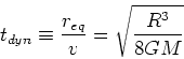
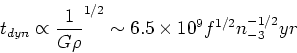
We can now compute an approximate turnaround time, i.e., the time when perturbation reaches max radius as

$$t(R_{max})\propto ({R_{max}^3\over M})^{1/2} \propto \rho^{-1/2}$$

In other words, the turnaround time depends on the density, not the mass. All lumps of a given density at a given epoch collapse at same time.

Consider growth of density. At early times we can derive from linear perturbation theory:

$$\delta \sim {R\over R_{max}}\propto a$$

and, in terms of overdensity, the turnaround time is

$$t(R_{max}) \propto \delta^{-3/2}$$

Lumps of higher overdensity collapse first. This growth rate, however, only applies to the linear regime.

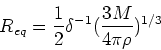
If there were no perturbations on a smaller scale, the perturbation at a given scale would collapse back to zero radius, i.e. infinite density. For spherical perturbation, one can compute ``linear perturbation overdensity'' when this occurs, and find that collapse happens at $\delta=1.69$ for $\Omega=1$, slightly lower for $\Omega<1$.

However, if there's perturbations on smaller scales, these cause random velocities to be generated, and perturbation settles into equilibrium configuration given by virial theorem:

$$E = T_{eq} + V_{eq} = V_{max}$$

$$2T_{eq} + V_{eq} = 0$$

giving

$$T_{eq} = -V_{max}$$

$$V_{eq} = 2 V_{max}$$

where $V$ is potential energy

$$V_{eq} = -{GM\over R_{eq}} = -{2GM\over R_{max}}$$

so

$$R_{eq} = {R_{max}\over 2}$$

Velocity dispersion

$$v^2\sim {2GM\over R}$$

Dynamical time

$$t_{dyn}\equiv {r_{eq}\over v} = \sqrt{R^3\over 8GM}$$

In terms of overdensity using $\delta \propto R/R_{max}$ and $r\propto (M/\rho)^{1/3}$, we get

$$R_{eq} = {1\over 2} \delta^{-1} ({3M\over 4\pi\rho})^{1/3}$$

$$v = \delta^{1/2}G^{1/2} M^{1/3} ({32\pi\rho\over 3})^{1/6}$$

$$t_{dyn} = \delta^{-3/2} ({3\over 32\pi G\rho})^{1/2}$$

These show that if you know the epoch ($\rho$), $\delta$, and mass, you can get the final equilibrium state.

In reality, the analytical treatment may be of limited applicability, because real perturbations aren't spherical.

Distribution of overdensities in the Universe

So now the next question is what is the distribution of overdensities as a function of mass in the Universe? Usually convenient to express this in Fourier space, with Fourier coefficients $\delta_k$:

$$\delta_k = {1\over V}\int d^3x \delta(x)e^{ik\dot x}$$

Generally, many theories (e.g. inflation) predict that $\delta_k \propto D(t) k^n$ initially, and that the coefficients have random and independent phases, i.e. a Gaussian field. $D(t)$ is the growth rate just discussed, which is a function of the cosmological model. Note also that the inital spectrum may be modified by physical processes in the Universe, as discussed below, so the actual power spectrum has a logarithmic slope that changes with wavenumber, but first let's consider some simple results for a single power law (which will be roughly applicable to the real case over limited ranges of scales).

The mean square fluctuation in a sphere of comoving radius R is

$$<({\Delta M\over M})^2> = \int d^3k W(kR)^2 \delta_k^2$$

where $W(kR)$ is the window function, which corresponds in this case to the Fourier transform of a function which is equal to $3/(4\phi R^3)$ for $x<R$ and zero everywhere else. For a power law perturbation spectrum,

$$<({\Delta M\over M})^2> \propto D^2 R^{-3-n} \propto M^{-1-n/3}$$

From this, once can see that if $n\geq -3$, then small scales collapse first, i.e. hierarchical clustering.

We can derive the characteristic mass which is going nonlinear at any epoch by setting ${\Delta M\over M} = 1$ for a general power law spectrum, and find

$$M_*(t) \propto D(t)^{6/(3+n)}$$

For $\Omega=1, D \propto a \propto (1+z)$, and we have

$$M_*(t) \propto (1+z)^{-6/(3+n)}$$

For a power law spectrum, clustering is ``self-similar''; at any given epoch clustering looks the same but at a different scale. However, most cosmological models are not pure power laws. Also, remember this is just for dissipationless collapse. These simple analytics are for spherical collapse - which is simpler than what really happens!

What is the fluctuation spectrum for the Universe? One can derive expression for the potential from above

$$<\Delta\Phi> \propto {G\Delta M\over a R} \propto M^{(1-n)/6}$$

and one sees that for $n=1$, potential is scale invariant. This is what is suggested by most inflationary models, and is called the Harrison-Zeldovich spectrum. However, this spectrum gets modified by subsequent physical processes.

First, the universe is not composed of a single species of matter; it is certainly composed of at least photons and baryons, and likely composed of at least one species of dark matter. Since the radiation density declines at a different (faster) rate than matter, at early times, the density of the universe is dominated by radiation; matter perturbations will grow at a different rate during that time.

Critical times: epoch of matter-radiation equality, epoch of recombination, epoch of horizon crossing, epoch at which dark matter becomes non-relativistic

A critical time for the growth of a perturbation is the epoch at which the perturbation ``crosses'' the horizon, i.e. the epoch at which there is sufficient time for causal contact across the entire population. Perturbations grow before this time, but the behavior requires a good understanding of general relativity and gauge theories. Small perturbations cross the horizon before large ones.

After horizon crossing, perturbations can begin to grow as described above. However, perturbations crossing the horizon before matter-radiation equality have slower growth. In addition, even after the universe becomes matter dominated, radiation can be important if the matter is ionized, because in that case it is coupled to the radiation via Thompson scattering. During this time, perturbations can be erased as photons diffuse out of the perturbation, a process known as ``Silk damping''. So baryon fluctuations can't really start to grow until after recombination.

For dark matter particles, the growth of their perturbations is affected by their random thermal motions; if these are large, they can prevent growth from occurring. The random thermal motions are related to the mass of the dark matter particles. Since we don't know what this is, dark matter is generically lumped into ``cold'' or ``hot'' dark matter. Observations of large scale structure suggest that the dark matter is ``cold''. For dark matter particles, perturbations are damped out if the velocities are substantial; this is called ``free-streaming''.

Summary: perturbations grow at different rate before horizon crossing, and smaller scales cross horizon first. In addition, smallest scales which cross horizon when radiation dominates hardly grow at all until matter dominates. For baryonic matter, growth is further suppressed until recombination. For hot dark matter candidates, growth is surpressed until particles become nonrelativistic.

Growth of perturbations plot. Final power spectrum plot.

Properties of halos

For a given cosmological model, we are interested in calculating the number of ``galaxies'' as a function of time and mass. Given a Gaussian field specified by the fluctuation spectrum, one can calculate the fraction of points surrounded by sphere R in which mean density exceeds some value. Press and Schecter suggested that if one adopted the linear overdensity at collapse of a spherical perturbation (1.69) one might associate this fraction with the fraction of particles which are part of nonlinear lumps with mass exceeding M. This suggestion, with some additional fudges, gives rise to the Press-Schecter formalism, which can be used to estimate the number of collapsed objects as a function of mass at any given time.

Given reasonable evidence for hierarchical clustering, we know that merging will be an important physical process. Consequently, it's of great utility to be able to analytically predict certain merging characteristics from a given fluctuation spectrum. A way of doing this was suggested by Bond et al and Lacey and Cole which is being fairly widely used in semi-analytic models of galaxy formation. The idea is, like for Press-Schecter, to find a prescription for identifying whether any given point is part of a nonlinear lump which one might associate with a galaxy halo. The scheme developed is as follows: for a given realization of the density field, smooth the field with filters of increasingly larger size, and compute the mean overdensity for each smoothing size. Associate the point with the mass of the largest smoothed region in which the mean overdensity exceeds some critical value, e.g., the linear spherical collapse overdensity. For appropriate choice of smoothing function, the mean overdensity as a function of smoothing size is exactly a Brownian random walk - for other window function, it's approximately random.

Can do this for any point in time by growing realization according to linear growth law. In practice, it's convenient to think about a single time-independent realization along with a threshold overdensity which decreases with time. Looking at random walk in such a picture gives a semi-analytic merging history (Lacey and Cole Fig 1). The nice thing about this formalism is that it allows one to calculate analytic expressions for a variety of interesting quatities: the probability than an object with given mass with merge with an object of some other mass as a function of time, the probability that an object of some mass will be included as part of an object of a larger mass at some later time, the distribution of formation times of objects with given mass, the distribution of survival times of objects, etc. Examples: merger rate (LC Fig 3 and Fig 4): mergers with small halos dominate numerically, but mass accretion rate is dominated by mergers with halos of higher mass. Survival time (LC Fig 5): small halos can survive a long time (wide distribution of survival times), but big halos are unlikely to - they have a much narrower distribution. Halo formation times (definition: a halo forms when it has accreted half of it's current mass) (LC Fig 6 and Fig 10): small halos form earlier.

Assess truth of such semi-analytics through N-body simulations. Find that assumption of associating single particle with halo isn't good, but statistical association is good! Discussion of numerical techniques and limitations.

Properties of dark matter halos

One final piece of information is needed for us to proceed with a model of galaxy formation, which is the distribution of matter within a given lump. A simple approximation which is found via numerical simulations to be poor, is to take it to be an isothermal sphere, with $\rho \propto r^{-2}$, out to the virial size of the lump. From numerical simulations, it appears that all hierarchical models produce halos with a characteristic density profile, known as the Navarro, Frenk, and White (NFW) profile, which has $\rho \propto r^{-1}$ in the inner regions, and $\rho\propto r^{-3}$ in the outer regions.

Note that this density profile may be further affected by the presence of baryons within the halo, as they collapse further (via dissipation) and then can act to gravitationally compress the dark matter halo (adiabatic compressions).

Dissipation

To compare with real observable galaxies, we need to consider dissipation. Cooling of gas allows baryonic matter to collapse further within a virialized halo, and this collapsed gas should correspond to observable galaxies. For gas to cool within a dark halo, the cooling time must be less than the crossing time, otherwise cooling will not occur. For a uniform cloud, the cooling time is given by:

$$t_{cool} = {3/2 nkT\over n^2 \Lambda(T)} = 6.6 \times 10^9 {T_6\over n_{-3} \Lambda_{-24}} yr$$

where $n_{-3}$ is the density in units of $10^{-3} cm^{-3}$ and $\Lambda_{-24}$ is the cooling in units of $10^{-24} ergs cm^3 s^{-1}$. $\Lambda_{-24}=1$ is roughly the minimum cooling rate for a primordial plasma at $T>10^4$ K. The dynamical time is given by

$$t_{dyn} \propto {1\over G\rho}^{1/2} \sim 6.5\times 10^9 f^{1/2} n_{-3}^{-1/2} yr$$

where $f$ is the gas fraction of a cloud. Seting the two time scales to be equal gives

$${T_6\over \Lambda_{-24}} \sim f^{1/2} n_{-3}^{1/2}$$

which, with a crude appoximation for the cooling curve, is

$$T_6^{3/2} f^{-1/2} n_{-3}^{-1/2} \approx 2.5$$

At higher densities and lower temperature, the cooling time is shorter.

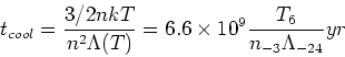
From the virial theorem, the relation between mass, temperature and density of a cloud is given by:

$$M_g = 1.2\times 10^{13} T_6^{3/2} f^{3/2} n_{-3}^{-1/2}$$

for $M_g$ in solar masses. Hence, our cooling criterion suggests that dissipational collapse will occur only for objects with

$$M_g \mathrel{\vcenter{\offinterlineskip \hbox{$<$} \kern 0.3ex \hbox{$\sim$}}}3\times 10^{13} f^2 \equiv f M_{lim}$$

where $M_{lim}$ is the limiting dark matter halo mass. Note that for small $f$, this roughly corresponds to galaxy masses!

One can proceed with this crude defintion of galaxies. If one identifies galaxies as all objects at a given time with $M<M_{lim}$, one can use the Press-Schecter formalism to derive the relative number of galaxies as a function of mass and epoch, i.e., a luminosity function. However, a problem arises. If all halos under the limiting mass turn into galaxies, one finds that at early times almost all of the mass is in such halos, so everthing turns into small galaxies early, and no gas is left to form big galaxies later! This has been called the cooling catastrophe. It's actually not so bad because the smallest halos are too cool to cool effectively and so might survive. However, it seems likely that some mechanism is needed to reduce the efficiency of galaxy formation.

A common proposal is that energy input from supernovae ejects gas from systems before it all turns into stars. Presumably, such an effect would work more effectively for systems with lower binding energy. If one postulates that some fraction of the gas mass is ejected with is proportional to the binding energy (which is $\propto v^2$), then one can derive a revised luminosity function. Using Press-Schecter, White and Rees derived such a relation and found that they could derive a Schecter-like form for the galaxy luminosity function. This is very encouraging! However, they derived a faint end slope of $(n-13)/(7-n)\sim -1.6$, which is considerably steeper than the observed value. Note that this contains no estimate for merging, however.

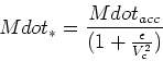
This whole cooling argument is quite crude, however, as it doesn't even account for the distribution of gas within a halo and the corresponding realization that the cooling time is a function of location. In fact, the inner parts of halos cool rapidly, and the cooling radius gradually moves out as a function of time. Given this, we can estimate the rate at which gas accretes onto an existing halo, which is a prerequiste for a star formation rate. The maximum accretion rate is the rate at which is halo is growing out of the surrounding material, and is given by

$$M^._{infall} = {0.15fV_c^3\over G}$$

However, if the cooling time in the outer halo is long, then material can only accrete in a slower cooling flow. This rate is given by

$$M^._{cool} = {3\over 4} f H_0 (1+z)^{3/2} {V_c^2r_{cool}\over G}$$

At a given $V_C$, cooling is more efficient at higher redshift and for larger gas fraction. The rate of accretion will be the smaller of the two rates: if the cooling time is shorter than the infall time, the infall rate limits the rate of accretion, if the accretion time is shorter, than cooling limits the accretion. Small halos are infall limited, large halos are cooling limited (white and frenk Fig 2).

Note that detailed cooling for galaxy formation is sensitive to metallicity, since critical temperature regime is where cooling is very sensitive to metallicity. This requires some model for chemical enrichment.

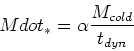
Finally, to model galaxy formation, we need to estimate how much of the infalling gas turns into stars, and account for the feedback from star formation. This is required to prevent the cooling catastrophe. A variety of scenarios have been suggested. At a minimum, we require a process which keeps too much gas from cooling. At a maximum, we might have a scenario in which gas in a halo is expelled entirely. Generally, supernovae is the mechanism invoked to inject energy. Unfortunately, it is very poorly understood with what efficiency energy is deposited. It can be parameterized by:

$${dE\over dt} = \epsilon Mdot^2_*$$

where $Mdot_*$ is the rate at which stars form. The minimum requirement is that this energy balance the energy associated with the dissipational losses for the component of the matter which does not form stars. This gives

$$\epsilon Mdot^2_* = (Mdot_{acc} - Mdot_*) V_c^2$$

where $Mdot_{acc}$ is the smaller of the accretion rate or the cooling rate. One can then solve for the star formation rate:

$$Mdot_* = {Mdot_{acc} \over (1+{\epsilon\over V_c^2})}$$

One then might consider whether to distribute such star formation uniformly over time or in a bursting fashion. WF Fig 3, SF higher at earlier epochs but note this doesn't have information about abundance of halos.

Alternatively, one might wish to allow some fraction of the cold gas to stay in the form of cold gas, i.e., not form stars. To do this one would need to assume some actual star formation law, such as the Kennicutt law. A very simple parameterization is to take

$$Mdot_* = \alpha {M_{cold}\over t_{dyn}}$$

where $\alpha$ is a free parameter, and $t_{dyn}$ is a characteristic dynamical time scale for the galaxy. One can then include feedback with some assumed energy per supernovae and number of supernovae given an IMF and the star formation rate. The numbers here are also very uncertain, so the feedback rate must also generally be considered to be a free parameter.

Once one decides on a star formation prescription, one can calculate actual brightnesses and colors as a function of time for each galaxy using stellar population synthesis models.

Finally, one needs to consider how to handle galaxies inside of halos which merge over time. Since these are in the centers of the potential wells, it's likely that the individual galaxies will not merge as fast as halos merge. A simple approximation to make is that all individual galaxies survive during a halo merging event, but that galaxies merge as time proceeds by the process of dynamical friction. This case can be parameterized as a merging rate proportional to the dynamical friction timescale for each galaxy, with a proportionality constant which is a free parameter to allow for uncertainties in orbit radii, etc. The simplest model just defines the most massive galaxy in a halo merger event to be the dominant galaxy, while all other galaxies are satellites which can eventually merge with the dominant galaxy, but not with each other. This is clearly a fairly crude approximation. One also needs to consider what happens to gas as it falls into a halo which has several galaxies in it; again, a simple, crude assumption is to have all of this gas go to the dominant galaxy, so star formation in satellite galaxies just dies out as their gas is depleted and is not replenished. This simple picture actually reproduces many features of observed galaxies! In addition, one can add features which allow all of the cold gas to turn into stars at the time of a merger to simulate starbursts, etc.

It's now possible to combine all of the aspects we've discussed into a coherent model for galaxy formation which might be compared with real galaxies. The different components are: 1) an estimate of the abundance of halos and merging rate as a function of mass and time, from PS or excursion set calculations given a cosmological model, 2) a cooling model for star formation inside of halos, 3) a model for how to handle merging of galaxies, 4) a prescription for how to assign morphologies to galaxies. For the following discussion, I am going to describe models constructed by Kauffmann, Guideroni, and White. They choose to identify ellipticals/bulges with galaxies that merge with comparable masses, with the critical ratio, $f_{ellip}$ as a free parameter. Their models, which are comparable with other models, then have the following free parameters: efficiency of star formation, efficiency of feedback, parameter for dynamical friction merging of galaxies, parameter for what to identify as spheroidal systems, cosmological parameters ($\Omega$, $\Omega_b$, $h$, normalization, $\Lambda$, etc.).

Generally Kauffmann et al have been considering CDM models. They proceed as follows. First they identify halos which have $V_c = 220$ km/s, for which they want to reproduce quantities observed for the Milky Way and its companions. First, they adjust the star formation and feedback efficiency to make the dominant galaxies within such halos match the brightness and neutral gas content of the Milky Way. As the star formation efficiency is increased, the galaxy gets brighter. As both star formation and feedback are increased, more cold gas is lost. So one can tune both parameters to match the observed quantities. Then one can look at the luminosity function of objects within the halo, corresponding to the MW and its companions. One finds that the model has far too many low mass neighbors if no galaxy merging is included (KWG Fig 1). If merging is included one can bring down the number of galaxies, but it brings down the number of brighter neighbors faster than fainter neighbors, so it also does not match the observations well. They are able to get a match only by inhibiting galaxy formation in small halos. There are plausible mechanisms for doing this, such as background ionization at early epochs from quasars, or possibly from more extreme feedback in smaller halos. KWG get reasonable agreement by inhibiting SF in halos with $V_c<150$ km/sec at $1.5<z<5$. They then compare colors of objects with the observations (KWG Fig 2). Generically, the hierarchicial clustering models predict redder colors for lower mass galaxies. This is understandable, since SF is turned off when objects merge in the model, so only the largest objects have ongoing star formation, and hence blue colors. The general trend is observed in real galaxies, but there's a conflict for the dominant galaxies, which are generally too blue in the models. However, note that the models don't have dust or chemical enrichment, both of which might make for redder objects.

One can then proceed to apply the model to other objects. Kauffmann et al compare with the Virgo cluster, and find reaonable agreement with the observed luminosity function for the same parameters (KWG Fig 3), except that they form a central galaxy which is much brighter than M87; to avoid this, they have to put in an ad hoc modification which turns off star formation in very massive halos. The models also approximately predicts the right percentages of E/S0 galaxies as a function of magnitude (KWG Fig 4).

The model can also be used to predict a Tully-Fisher relation (KWG Fig 7), and reasonable agreement can be found. In this model, the TF relation arises from the relation between star formation and feedback, and the good agreement arises partly because the model is normalized to the Milky Way.

A significant problem with the model is that the mean luminosity density of the model is roughly a factor of two higher than that of the real universe. This comes because there are too many faint galaxies. This may be a result of the cosmological model adopted.

One can use the same model to see if one can understand the faint blue galaxies. This sort of model naturally predicts a steepening of the LF at higher redshifts even without merging, since star formation is turned off in smaller galaxies as their halos merge with larger ones. Reasonable fits can be found to the observational data, especially for models which can reduce the number of faint galaxies at present.

Finally, lets consider the issue of elliptical galaxy formation. In the model, we form spheroidal systems by roughly equal mass mergers. If this merged galaxy is the dominant galaxy, it will quickly accrete gas and become a ``spiral''. However, if its halo merges again with a more massive halo, the elliptical can passively evolve. The question is whether such a model for elliptical formation is consisent with the lack of spread in the Mg-$\sigma$ relation. One finds that in clusters, the luminosity weighted mean age of the ellipticals are all pretty old (Kaffmann MN 281, 487, fig 1), but that in the field, brighter E's are younger (Fig 2). Interpretation is clear: in field galaxies continue to accrete gas. This makes field ellipticals quite different from cluster ellipticals; cluster Es have stopped accreting gas and will evolve passively, but field Es continue to accrete and may turn into spirals! The models are consistent with the lack of scatter observed in elliptical colors or line strengths. However, the model predicts that this scatter will get significantly larger at $z>1$.

Numerical models of galaxy formation

(Klypin).

N-body codes: direct, PM, PPPM, ART. Size and resolution (spatial and temporal)

Gas dynamics: SPH vs. hydro codes.

Stellar physics...